Quick Start#

Data Download#

seafog comes with a lot functions to download data from various sources. Here we use function pgm_find_data to download satellite data from Kochi University and function goos_sst_find_data to download NEAR-GOOS SST data from Japan Meteorological Agency. Both of these functions will return paths of datas they download. You can go to page Module to handle PGM satellite data and page Module to handle NEAR-GOOS SST data for more information about them.

main.py#

from pprint import pprint
from seafog import pgm_find_data, goos_sst_find_data

fog_date = "2021-03-25 03:00"   # UTC time
pgm_save_path = "data/pgm"      # the dir store PGM data
goos_save_path = "data/goos"    # the dir store NEAR-GOOS data

IR1, IR4, VIS, table = pgm_find_data(fog_date, pgm_save_path)
sst = goos_sst_find_data(fog_date, goos_save_path)

pprint([IR1, IR4, VIS, table])
pprint(sst)

output#

['data/pgm/HMW821032503IR1.pgm',
 'data/pgm/HMW821032503IR4.pgm',
 'data/pgm/HMW821032503VIS.pgm',
 'data/pgm/HMW821032503CAL.dat']
'data/goos/re_mgd_sst_glb_D20210325.txt'

As you can see, all of these data are shipped in PGM or TXT format, which are not easy to parse. seafog provides pgm_parser and goos_sst_parser to reads these data and converts them to a xarray.DataArray object.

main.py#

from seafog import pgm_parser, goos_sst_parser

IR1 = pgm_parser(IR1, table, data_type="IR1")
IR4 = pgm_parser(IR4, table, data_type="IR4")
# use built in table to read VIS data
VIS = pgm_parser(VIS, "", data_type="VIS-b")

sst = goos_sst_parser(sst)

print(IR4)
print(sst)

Detect seafog#

Interpolate and mask data#

Because the resolution of satellite data and SST is different, we need to interpolate them to the same resolution at first. NaN values in SST will be removed because they can affect the interpolation, so we have to mask land values after interpolating. Let’s interpolate the data to a resolution of 0.0416°, which is around 4-km.

main.py#

import numpy as np
from seafog import mask_land

# set nan in sst to -10
sst = sst.fillna(263.16)
latitude = np.arange(30, 42, 0.0416)
longitude = np.arange(115, 130, 0.0416)
# interpolate and mask data
IR1 = IR1.interp(coords={'latitude': latitude, 'longitude': longitude})
IR4 = IR4.interp(coords={'latitude': latitude, 'longitude': longitude})
VIS = VIS.interp(coords={'latitude': latitude, 'longitude': longitude})
sst = sst.interp(coords={'latitude': latitude, 'longitude': longitude})
# mask sst value on land
sst = mask_land(sst)

print(IR4)
print(sst)

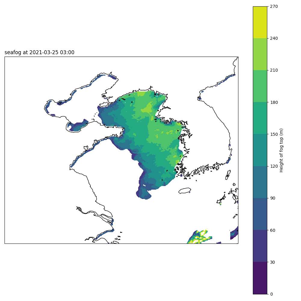
Calculate marine fog area and the height of fog top#

We will use detect_seafog.daytime_seafog to calculate marine fog area and the height of its top at daytime.

main.py#

import matplotlib.pyplot as plt
from cartopy import crs
from seafog import detect_seafog

detect_seafog.IR_sst_diff_range = (0, 35)
seafog = detect_seafog.daytime_seafog(fog_date, IR1, IR4, VIS, sst)

fig = plt.figure(figsize=(10, 10))
proj = crs.PlateCarree()
ax = fig.add_subplot(111, projection=crs.PlateCarree(central_longitude=180))
im = ax.contourf(seafog['longitude'], seafog['latitude'], seafog, levels=np.arange(0, 300, 30), transform=proj)
ax.coastlines()
ax.set_title(f"seafog at {fog_date}", loc='left')
cbar = fig.colorbar(mappable=im)
cbar.set_label("Height of fog top (m)")
plt.show()

Quick Start#

Data Download#

Detect seafog#

Interpolate and mask data#

Calculate marine fog area and the height of fog top#

This Page